In my two previous posts, we saw how we can perform Linear Regression using TensorFlow, but I’ve used Linear Least Squares Regression and Cholesky Decomposition, both them use matrices to resolve regression, and TensorFlow isn’t a requisite for this, but you can use more general packages like NumPy.
One of the most common applications of TensorFlow is training models by reducing loss function by backpropagation, and training the model by batches, this allow us to optimize the Gradient Descent and converge to solution.
Advantage: It allow us to use big amounts of data, and TensorFlow process it by batches.
Disadvantage: Solution is not so precise as if we use Linear Least Squares or Cholesky Decomposition.
In the following example I’ll use Iris data from scikit-learn (Sepal Length vs Pedal Width seem to have a linear relationship in the form y = mx + b), and L2 loss function:
import matplotlib.pyplot as plt
import numpy as np
import tensorflow as tf
from sklearn import datasets
sess = tf.Session()
iris = datasets.load_iris()
x_vals = np.array([x[3] for x in iris.data])
y_vals = np.array([x[0] for x in iris.data])
learning_rate = 0.25
batch_size = 25
x_data = tf.placeholder(shape=(None, 1), dtype=tf.float32)
y_target = tf.placeholder(shape=(None, 1), dtype=tf.float32)
m = tf.Variable(tf.random_normal(shape=[1, 1]))
b = tf.Variable(tf.random_normal(shape=[1, 1]))
model_output = tf.add(tf.matmul(x_data, m), b)
loss = tf.reduce_mean(tf.square(y_target - model_output))
init = tf.global_variables_initializer()
sess.run(init)
my_opt = tf.train.GradientDescentOptimizer(learning_rate=learning_rate)
train_step = my_opt.minimize(loss)
loss_vec = []
for i in range(100):
rand_index = np.random.choice(len(x_vals), size=batch_size)
rand_x = np.transpose([x_vals[rand_index]])
rand_y = np.transpose([y_vals[rand_index]])
sess.run(train_step, feed_dict={x_data: rand_x, y_target: rand_y})
temp_loss = sess.run(loss, feed_dict={x_data: rand_x, y_target: rand_y})
loss_vec.append(temp_loss)
if (i + 1) % 25 == 0:
print('Step #' + str(i + 1) + ' A = ' + str(sess.run(m)) + 'b = ' + str(sess.run(b)))
print('Loss = ''' + str(temp_loss))
[m_slope] = sess.run(m)
[y_intercept] = sess.run(b)
best_fit = []
for i in x_vals:
best_fit.append(m_slope * i + y_intercept)
plt.plot(x_vals, y_vals, 'o', label='Points')
plt.plot(x_vals, best_fit, 'r-', label='Linear Reg.', linewidth=3)
plt.legend(loc='upper left')
plt.title('Sepal Length vs Pedal Width')
plt.xlabel('Pedal Width')
plt.ylabel('Sepal Length')
plt.show()
plt.plot(loss_vec, 'k-')
plt.title('L2 Loss')
plt.xlabel('Batches')
plt.ylabel('L2 Loss')
plt.show()
>> Step #25 A = [[0.90450525]]b = [[4.513903]]
>> Loss = 0.26871145
>> Step #50 A = [[0.94802374]]b = [[4.7737966]]
>> Loss = 0.2799243
>> Step #75 A = [[1.1669612]]b = [[4.906186]]
>> Loss = 0.2010894
>> Step #100 A = [[0.84404486]]b = [[4.730052]]
>> Loss = 0.15839271

Conclusion
As we can see in the graphic, the gradient descent tries to converge to solution, but it is not so precise as matrix operations for Linear Least Squares and Cholesky Decomposition.