Cholesky Decomposition for Linear Regression with TensorFlow

Several years have already passed since the onset of the Deep Learning boom. I have witnessed impressive achievements like ChatGPT and Midjourney, however, I am still amazed at how traditional methods like Cholesky decomposition remain extremely useful and efficient. Particularly, for tasks like Linear Regression, this method stands out due to its efficiency and speed in calculation.

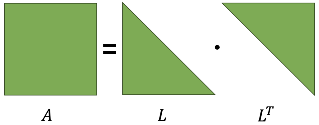
Even though Least Squares Linear Regression is straightforward and accurate, it can become inefficient when dealing with large matrices. Cholesky decomposition offers an alternative to solve these matrices effectively. This technique decomposes a matrix into two triangular matrices: a lower one (lower) and a transposed lower one (L and L^T), with which the original matrix is obtained, as illustrated in the following figure.

\begin{bmatrix} a_{11} & a_{12} & a_{13} & a_{14}\\ a_{21} & a_{22} & a_{23} & a_{24}\\ a_{31} & a_{32} & a_{33} & a_{34}\\ a_{41} & a_{42} & a_{43} & a_{44} \end{bmatrix}=\begin{bmatrix} l_{11} & 0 & 0 & 0\\ l_{21} & l_{22} & 0 & 0\\ l_{31} & l_{32} & l_{33} & 0\\ l_{41} & l_{42} & l_{43} & l_{44} \end{bmatrix}\cdot \begin{bmatrix} l_{11} & l_{21} & l_{31} & l_{41}\\ 0 & l_{22} & l_{32} & l_{42}\\ 0 & 0 & l_{33} & l_{43}\\ 0 & 0 & 0 & l_{44} \end{bmatrix}

The product of the multiplication of the two matrices is shown below:

A=\begin{bmatrix} {l_{11}}^{2} & l_{21}l_{11} & l_{31}l_{11} & l_{41}l_{11}\\ l_{21}l_{11} & {l_{21}}^{2}+{l_{22}}^{2} & l_{31}l_{21}+l_{32}l_{22} & l_{41}l_{21}+l_{42}l_{22}\\ l_{31}l_{11} & l_{31}l_{21}+l_{32}l_{22} & {l_{31}}^{2}+{l_{32}}^{2}+{l_{33}}^{2} & l_{41}l_{31}+l_{42}l_{32}+l_{43}l_{33}\\ l_{41}l_{11} & l_{41}l_{21}+l_{42}l_{22} & l_{41}l_{31}+l_{42}l_{32}+l_{43}l_{33} & {l_{31}}^{2}+{l_{32}}^{2}+{l_{33}}^{2}+{l_{44}}^{2} \end{bmatrix}

From this point on, each element is an equation from which the following is deduced:

A feature (or limitation) of Cholesky decomposition is that it only works on positive symmetric matrices.

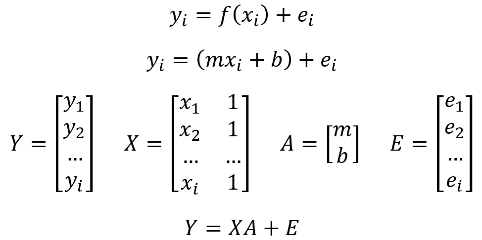
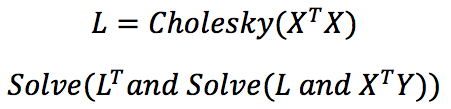
Finally, linear regression through Cholesky decomposition is analogous to Linear Least Squares, but reduced to solving a system of linear equations.

Cholesky Decomposition is already implemented in TensorFlow, PyTorch, or NumPy, however, you can review more details about Cholesky Decomposition.

import matplotlib.pyplot as plt
import tensorflow as tf
import numpy as np

# Generate data
x_vals = np.linspace(start=0, stop=10, num=100)
y_vals = x_vals + np.random.normal(loc=0, scale=1, size=100)

x_vals_column = np.transpose(np.matrix(x_vals))
ones_column = np.transpose(np.matrix(np.repeat(a=1, repeats=100)))
X = np.column_stack((x_vals_column, ones_column))
Y = np.transpose(np.matrix(y_vals))
X_tensor = tf.constant(X, dtype=tf.float64)
Y_tensor = tf.constant(Y, dtype=tf.float64)

# Perform computations
tX_X = tf.matmul(tf.transpose(X_tensor), X_tensor)
L = tf.linalg.cholesky(tX_X)
tX_Y = tf.matmul(tf.transpose(X_tensor), Y_tensor)
sol1 = tf.linalg.solve(L, tX_Y)
sol2 = tf.linalg.solve(tf.transpose(L), sol1)

# Extract coefficients
solution_eval = sol2.numpy()
m_slope = solution_eval[0][0]
b_intercept = solution_eval[1][0]

print('slope (m): ' + str(m_slope))
print('intercept (b): ' + str(b_intercept))

# Visualization
best_fit = []
for i in x_vals:
    best_fit.append(m_slope * i + b_intercept)

plt.plot(x_vals, y_vals, 'o', label='Data')
plt.plot(x_vals, best_fit, 'r-', label='Linear Regression', linewidth=3)
plt.legend(loc='upper left')
plt.show()

import matplotlib.pyplot as plt
import torch
import numpy as np

# Generate data
x_vals = np.linspace(start=0, stop=10, num=100)
y_vals = x_vals + np.random.normal(loc=0, scale=1, size=100)

x_vals_column = np.transpose(np.matrix(x_vals))
ones_column = np.transpose(np.matrix(np.repeat(a=1, repeats=100)))
X = np.column_stack((x_vals_column, ones_column))
Y = np.transpose(np.matrix(y_vals))
X_tensor = torch.tensor(X, dtype=torch.float64)
Y_tensor = torch.tensor(Y, dtype=torch.float64)

# Perform computations
tX_X = torch.mm(X_tensor.T, X_tensor)
L = torch.cholesky(tX_X)
tX_Y = torch.mm(X_tensor.T, Y_tensor)
sol = torch.cholesky_solve(tX_Y, L)

# Extract coefficients
m_slope = sol[0][0].item()
b_intercept = sol[1][0].item()

print('slope (m): ' + str(m_slope))
print('intercept (b): ' + str(b_intercept))

# Visualization
best_fit = []
for i in x_vals:
    best_fit.append(m_slope * i + b_intercept)

plt.plot(x_vals, y_vals, 'o', label='Data')
plt.plot(x_vals, best_fit, 'r-', label='Linear Regression', linewidth=3)
plt.legend(loc='upper left')
plt.show()

import matplotlib.pyplot as plt
import numpy as np

# Generate data
x_vals = np.linspace(start=0, stop=10, num=100)
y_vals = x_vals + np.random.normal(loc=0, scale=1, size=100)

x_vals_column = np.transpose(np.matrix(x_vals))
ones_column = np.transpose(np.matrix(np.repeat(a=1, repeats=100)))
X = np.column_stack((x_vals_column, ones_column))
Y = np.transpose(np.matrix(y_vals))

# Perform computations using Cholesky Decomposition
tX_X = np.dot(X.T, X)
L = np.linalg.cholesky(tX_X)
tX_Y = np.dot(X.T, Y)
sol = np.linalg.solve(L, tX_Y)
beta = np.linalg.solve(L.T, sol)

# Extract coefficients
m_slope = beta[0,0]
b_intercept = beta[1,0]

print('slope (m): ' + str(m_slope))
print('intercept (b): ' + str(b_intercept))

# Visualization
best_fit = []
for i in x_vals:
    best_fit.append(m_slope * i + b_intercept)

plt.plot(x_vals, y_vals, 'o', label='Data')
plt.plot(x_vals, best_fit, 'r-', label='Linear Regression', linewidth=3)
plt.legend(loc='upper left')
plt.show()

slope (m): 1.0830263227926582
intercept (b): -0.3348165868955632

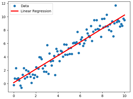
As you can see, this solution is very similar to Linear Least Squares, but this decomposition is sometimes much more efficient and numerically stable.

Tags: choleskylinear regressionmachine learningpythonpytorchtensorflow